Below are some notes I took while working through chapter 2 of my favorite Python machine learning textbook.
Artificial Neurons
- Define an activation function \(\phi(z)\) that takes a linear combination of certain input values x and corresponding weight vector w, where z is the so-called net input (\(z = w_1x_1 + \ldots + w_mx_m\)).
- Denote particular input sample as \(x^i\).
- In the perceptron algorithm, the activation function is a simple unit step function: \(\phi(z) = \begin{cases} 1 & z \geq \theta \\ -1 & otherwise \\ \end{cases}\)
- Simplify by bringing the threshold \(\theta\) into the weight vector via \(w_0 = -\theta\), and always set \(x_0 = 1\), so now: \(\phi(z) = \begin{cases} 1 & z \geq 0 \\ -1 & otherwise \\ \end{cases}\)
- Procedure: Perceptron Algorithm
- Init weights to 0 or small random numbers.
- For each training sample \(x^{(i)}\) perform:
- Compute the output (predicted class) value \(\hat{y}\) using the aforementioned step function.
- Simultaneously update all weights: \(\begin{align} w_j :&= w_j + \Delta w_j \\ \Delta w_j &= \eta \Big( y^{(i)} - \hat{y}^{(i)} \Big) x_j^{(i)} \end{align}\)
- Properties: Perceptron Algorithm
- Convergence only guaranteed if the two classes are linearly separable, and learning rate \(\eta\) sufficiently small.
- If the two classes can’t be separated by a linear decision boundary, can do one or both of the following:
- Set a maximum number of passes over the training dataset (epochs).
- A threshold number of tolerated misclassifications.
import numpy as np

class Perceptron(object):
    """ Perceptron classifier.

    Parameters
    ----------
    eta : float
        Learning rate (between 0.0 and 1.0)
    n_iter : int
        Passes over the training dataset.

    Attributes
    ----------
    w_ : 1d-array
        Weights after fitting.
    errors_ : list
        Number of misclassifications in every epoch.
    """
    def __init__(self, eta=0.01, n_iter=10):
        self.eta = eta
        self.n_iter = n_iter

    def fit(self, X, y):
        """ Fit training data.

        Parameters
        ----------
        X : {array-like}, shape = [n_samples, n_features]
            Training vectors, where n_samples is the number of samples and
            n_features is the number of features.
        y : array-like, shape = [n_samples]
            Target values.

        Returns
        -------
        self : object

        """
        # Initialize weight vector to zeros.
        # X.shape[1] returns the numer of features.
        self.w_ = np.zeros(1 + X.shape[1])
        self.errors_ = []

        for _ in range(self.n_iter):
            errors = 0
            for xi, target in zip(X, y):
                update = self.eta * (target - self.predict(xi))
                self.w_[1:] += update * xi
                self.w_[0] += update
                errors += int(update != 0.0)
            self.errors_.append(errors)
        return self

    def net_input(self, X):
        """ Calculate the net input. (i.e. do dot prod)"""
        return np.dot(X, self.w_[1:]) + self.w_[0]

    def predict(self, X):
        """ Return class label after unit step. """
        # Evaluates if (the single number) self.net_input(X) is >= 0.0, and
        # if it is, returns 1, otherwise returns -1.
        return np.where(self.net_input(X) >= 0.0, 1, -1)
Training a perceptron model on the Iris dataset
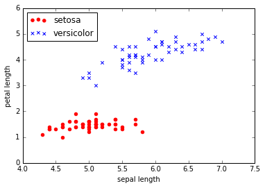
- Features considered: sepal length, petal length.
- Flower classes: Setosa, Versicolor.
- Procedure:
- Use the pandas library to load the Iris dataset into a DataFrame object.
- Extract the first 100 class labels.
- Visualize input data features/label in a scatter plot.
- Train the perceptron algorithm on the Iris data subset.
# Step 1 : Load datset into a pandas DataFrame.
import pandas as pd
df = pd.read_csv('https://archive.ics.uci.edu/ml/'
                'machine-learning-databases/iris/iris.data', header=None)
# Print the last five lines.
# First feat column = sepal length
# Third feat column = petal length
df.tail()
| 0 | 1 | 2 | 3 | 4 | |
|---|---|---|---|---|---|
| 145 | 6.7 | 3.0 | 5.2 | 2.3 | Iris-virginica |
| 146 | 6.3 | 2.5 | 5.0 | 1.9 | Iris-virginica |
| 147 | 6.5 | 3.0 | 5.2 | 2.0 | Iris-virginica |
| 148 | 6.2 | 3.4 | 5.4 | 2.3 | Iris-virginica |
| 149 | 5.9 | 3.0 | 5.1 | 1.8 | Iris-virginica |
%matplotlib inline
# Steps 2 and 3 : Extract our (simpler) desired subset and plot.
import matplotlib.pyplot as plt
import numpy as np

# Extract the first 50 Iris-Setosa and 50 Iris-Versicolor flowers, respectively.
# Syntax: df.iloc returns (index, value(s)) list, where
# (1) the 0:100 means "Get the first 100 data frame entries, and
# (2) the 4 means "only the (zero-indexed) 4th column of those entries, specifically.
# (3) .values means we only return the values, not their original indices.
y = df.iloc[0:100, 4].values
# Convert the class labels to integer labels: Setosa(-1), Versicolor(1).
y = np.where(y == 'Iris-setosa', -1, 1)

# Similarly, store the two features in X, obtained by
# getting the 0th and 2nd columns from the df object.
X = df.iloc[0:100, [0, 2]].values

# _______ Plotting _______
# Plot setosas in 2D feature space and mark with circles.
plt.scatter(X[:50, 0], X[:50, 1], color='red', marker='o', label='setosa') # X[row_indexer, col_indexer]
# Plot setosas in 2D feature space and mark with circles.
plt.scatter(X[50:100, 0], X[50:100, 1], color='blue', marker='x', label='versicolor')
plt.xlabel('sepal length')
plt.ylabel('petal length')
plt.legend(loc='upper left')
plt.show()
# Step 4 : Train the perceptron and make plots.
ppn = Perceptron(eta=0.1, n_iter=10)
ppn.fit(X, y)
plt.plot(range(1, len(ppn.errors_) + 1), ppn.errors_, marker='o')
plt.xlabel('Epochs')
plt.ylabel('Number of misclassifications')
plt.show()
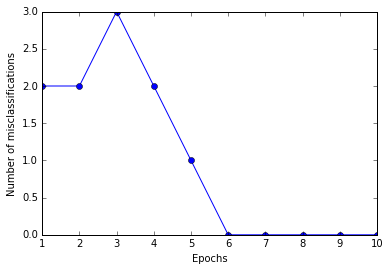
# Figure above shows that convergence occurred after 6th epoch.
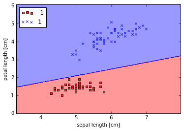
# Implement awesome visualization function for decision boundaries of 2D datasets.
from matplotlib.colors import ListedColormap

def plot_decision_regions(X, y, classifier, resolution=0.02):
    # Setup marker generator and color map.
    markers = ('s', 'x', 'o', '^', 'v')
    colors = ('red', 'blue', 'lightgreen', 'gray', 'cyan')
    cmap = ListedColormap(colors[:len(np.unique(y))])

    # Get the min/max (of each) feature values in the dataset.
    x1_min, x1_max = X[:, 0].min() - 1, X[:, 0].max() + 1
    x2_min, x2_max = X[:, 1].min() - 1, X[:, 1].max() + 1

    # Syntax overview:
    # (1) np.arange(start, stop, step) // Note: step will be nx or ny in meshgrid comment below.
    # (2) np.meshgrid(x, y):
    # ----> Input: x, y are arrays of length (nx, ny) respectively.
    # ----> Returns: Two arrays, each with shape (ny, nx):
    # --------> xx1 = NY number of copies of the input array X.
    # --------> xx2 = NY number of arrays where the ith array is the ith y-value from input Y, NX times.
    xx1, xx2 = np.meshgrid(np.arange(x1_min, x1_max, resolution),
                          np.arange(x2_min, x2_max, resolution))

    # Assign class prediction on matrix grid of POSSIBLE (x1, x2) values (no real corresp with data yet).
    # np.ravel() is basically np.flatten() except doesn't make a copy, but rather keeps original in some sense.
    Z = classifier.predict(np.array([xx1.ravel(), xx2.ravel()]).T)
    Z = Z.reshape(xx1.shape)

    plt.contourf(xx1, xx2, Z, alpha=0.4, cmap=cmap)
    plt.xlim(xx1.min(), xx1.max())
    plt.ylim(xx2.min(), xx2.max())

    # Plot class samples.
    for idx, cl in enumerate(np.unique(y)):
        plt.scatter(x=X[y == cl, 0], y=X[y == cl, 1],
                    alpha=0.8, c=cmap(idx),
                    marker=markers[idx], label=cl)
# Draw a contour plot that maps different decision regions to different colors for each predicted class
# in the grid array.
plot_decision_regions(X, y, classifier=ppn)
plt.xlabel('sepal length [cm]')
plt.ylabel('petal length [cm]')
plt.legend(loc='upper left')
plt.show()
Adaptive linear neurons and the convergence of learning
- ADAptive LInear NEuron (Adaline): Uses a linear activation function, \(\phi(z=w^Tx) = w^Tx\), rather than the step-function used by the perceptron.
- Interesting bc lays groundwork for understanding more advanced ML algorithms.
- NOTE: Resulting output is identical to perceptron since the activation function is directly fed to a quantizer in order to predict the class label. The difference is that the weight updates use the raw output of the activation function \(\phi(z)\). See figure in page 33.
Minimizing cost functions with gradient descent
- Define an objective function that is to be optimized during the learning process.
- Is often a cost function that we want to minimize.
- For adaline, can define cost function \(J\) to learn the weights as the Sum of the Squared Errors (SSE) bw the calculated outcomes and the true class labels. \(J(\mathbf{w}) = \frac{1}{2} \sum_i \Big( y^{(i)} - \phi(z^{(i)}) \Big)^2\)
- Factor of 1/2 just added for convenience; makes gradient derivation easier.
- New gradient descent weight update: \(\mathbf{w} := \mathbf{w} - \eta \nabla J(\mathbf{w})\)
- Based on all samples in training set, which is why also referred to as batch gradient descent.
- When implementing, recognize that \(-\eta \frac{\partial J}{\partial w_j} = \eta \sum_i \Big( y^{(i)} - \phi( z^{(i)} ) \Big) x_j^{(i)}\)
# Implementation of ADALINE. (see perceptron class for more descriptive comments)
class AdalineGD(object):
    """ ADAptive LInear NEuron classifier. """
    def __init__(self, eta=0.01, n_iter=50):
        self.eta = eta
        self.n_iter = n_iter

    def fit(self, X, y):
        """ Learn the weights. """
        self.w_ = np.zeros(1 + X.shape[1])
        self.cost_ = []
        for _ in range(self.n_iter):
            # Output == np.array(all dot prods corresp. to all samples)
            output = self.net_input(X)
            # Obtain array of all differences y(i) - phi(z(i)) at once. J
            errors = (y - output)
            # Weight update. Note:
            # X.T.dot(errors) is sum of input x^i vecs multiplied by scalar difference y^i - phi(z^i).
            # So the weight vector is updated by summing over (samp_i predict err) * (sample i),
            # and thus each _individual_ weight is updated by (samp_i predict err) * (jth feat of samp i)
            self.w_[1:] += self.eta * X.T.dot(errors)
            self.w_[0] += self.eta * errors.sum() # sum bc. sum(x) == x^T * (vec of ones)
            cost = (errors**2).sum() / 2.0
            self.cost_.append(cost)
        return self

    def net_input(self, X):
        """ Returns vector of dot products between samples and current weights. """
        return np.dot(X, self.w_[1:]) + self.w_[0]

    def activation(self, X):
        """ Adaline activation is the identity function. """
        return self.net_input(X)

    def predict(self, X):
        return np.where(self.activation(X) >= 0.0, 1, -1)
# Plot the cost against the number of epochs for two different learning rates.
fig, ax = plt.subplots(nrows=1, ncols=2, figsize=(12, 6))

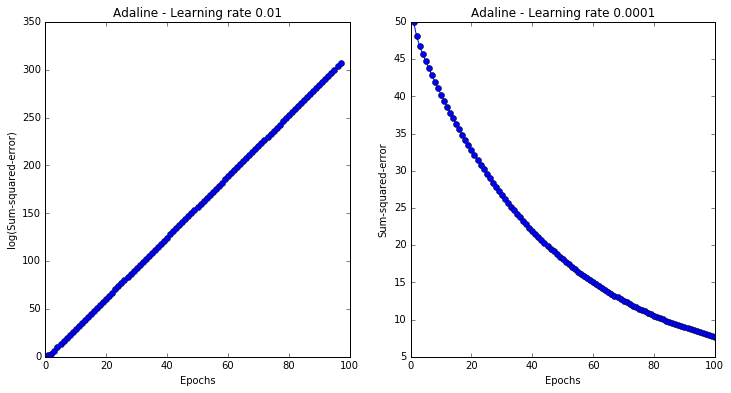
# High learning rate will overshoot the global minimum by so much each update, that it will end up
# on the other side of the parabola at a higher value, thus doing the opposite of minimizing basically.
ada1 = AdalineGD(eta=0.01, n_iter=100).fit(X, y)
ax[0].plot(range(1, len(ada1.cost_) + 1), np.log10(ada1.cost_), marker='o')
ax[0].set_xlabel('Epochs')
ax[0].set_ylabel('log(Sum-squared-error)')
ax[0].set_title('Adaline - Learning rate 0.01')

ada2 = AdalineGD(eta=0.0001, n_iter=100).fit(X, y)
ax[1].plot(range(1, len(ada2.cost_) + 1), ada2.cost_, marker='o')
ax[1].set_xlabel('Epochs')
ax[1].set_ylabel('Sum-squared-error')
ax[1].set_title('Adaline - Learning rate 0.0001')
plt.show()
Feature scaling for optimal performance (more in CH 3)
- Gradient descent can benefit from feature scaling.
- Here we use a feature scaling method called standardization which gives our data the property of a standard normal distribution.
- Mean of each feature centered at 0 and standard dev of 1 (for the given feature column).
- \[x'_j = \frac{x_j - \mu_j}{\sigma_j}\]
# Implement standardization with numpy methods 'mean' and 'std'.
X_std = np.copy(X) # read "X standardized"
X_std[:, 0] = (X[:,0] - X[:,0].mean()) / X[:,0].std()
X_std[:, 1] = (X[:,1] - X[:,1].mean()) / X[:,1].std()

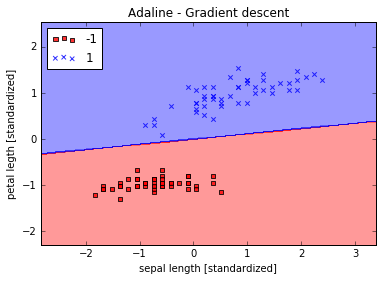
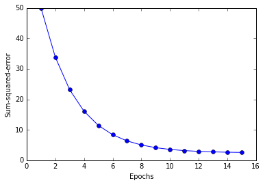
# Train the adaline again and see that is now converges with a learning rate of 0.01.
ada = AdalineGD(n_iter=15, eta=0.01).fit(X_std, y) # arg order doesn't matter??
plot_decision_regions(X_std, y, classifier=ada)
plt.title('Adaline - Gradient descent')
plt.xlabel('sepal length [standardized]')
plt.ylabel('petal legth [standardized]')
plt.legend(loc='upper left')
plt.show()

plt.plot(range(1, len(ada.cost_) + 1), ada.cost_, marker='o')
plt.xlabel('Epochs')
plt.ylabel('Sum-squared-error')
plt.show()
YESSS